Brownian motion is an important part of Stochastic Calculus. When you start developing quantitative trading strategies, pretty soon you will hit upon Brownian Motion. If you are interested in designing and developing algorithmic trading strategies than you should know stochastic calculus and Brownian motion. It will take some effort to learn stochastic calculus and Brownian motion. I am writing this post in an effort to help you in this regard. I will try to start from the beginning and then take you to the end of Brownian motion theory and show you how to apply it in modeling currency prices. Did you download this month copy of the Top Shelf Trader Magazine?
Days of traditional classic technical analysis are over. As a retail trader you are pitted against the world’s brightest minds working for hedge funds and big financial institutions. These big financial firms pay these MIT graduates salaries that are most of the time in six figures. These guys are known as quants. The job of these quants is to build quantitative trading strategies. So as a retail trader you are pitted against these big financial firms and their brilliant MIT graduates and vast resources at their disposal like super fast computers and super fast data feeds. Read this post on how to make 400 pips with a 12 pip stop loss.
Trading is a zero sum game. If you win, someone loses. If you lose, someone is grabbing your money. Most probably it is these big financial firms and their quants. It is as simple as that. if you want to win, then you will have to compete against these big firms and their quants. So trading is the ultimate game of mind against minds. As a retail trader, you are not competing against a single MIT graduate but thousands of them employed by these big firms with big pockets. You cannot see these people but they are their. FOMC monthly meeting is known to make the currency market highly volatile. Read this post on how I made 300 pips with FOMC meeting.
If you want to compete against these people than you should learn their methods. Just keep this in mind, Wall Street has the deep pockets to employ the best and the brightest minds that the world has to offer. Just do a job search and you can find how much these guys get paid by these big Wall Street firms. Now if you think that by playing with trendlines and fibonnaci ratios you will be able to defeat these people you are in for a shock. These guys use advanced quantitative methods in unearthing the inefficiencies in the market.
As said, they work with super fast computers. They have super fast price feeds that goes way beyond the open, high, low, close and volume data that we retail traders get. Call these people rocket scientists. Inside the firms that these rocket scientists work, superfast computers are at work 24/7 monitoring price and volume data tick by tick. They get their price data from vendors like Thomson Reuters that provides them 100,000 tick data per second databases. You must have heard of MATLAB. Most of the algorithmic trading strategies are developed using MATLAB.
Thomson Reuters and Bloomberg provide these big firms high speed news feed that has meta tags built into it. Algorithmic trading strategies use the meta tags in the news feeds to quantify the impact of the news on the markets.This is done in a few milliseconds and after that the algorithmic trading system starts executing the trades in less than a second of receiving the news. Compare this to yourself as a retail trader; When you receive the news, you can take 15-30 minutes to properly analyze it. Trading exotic pairs can be highly lucrative. Read this post on a USDTRY trade that made 1000 pips with 30 pip stop loss.
This was just a picture to tell you what is your competition. Should you lose heart? No, not at all. Keep reading my blog and I will show you how you can outsmart these people at their own game by doing exactly what they are doing. Just keep this in mind, traditional technical analysis no longer works. These guys have the advantage and they can see price action changing a lot earlier than you. So you need a method that can help you take away their advantage.Just know this. Markets are dominated by these big financial firms and super talented quants and you are competing against them as a retail trader, If you want to win than you will have to compete against these super talented people seriously.
How To Value An Options Contract?
Financial markets are ruled by Brownian Motion. Suppose you want to price an options contract on a currency pair or for that matter a stock. Things are uncertain here. We don’t know the payoff of the options contract at expiry since we don’t know what will be the price of the underlying instrument on which the options contract has been written. If it is a currency pair or if it is a stock, things are highly uncertain and we should have a method that tells us how to value the options contract before we buy it. If we don’t know how to price an options contract we can end up paying too high a price for the contract..
Suppose the expiry date or the payoff date is T. Suppose the price of the currency pair or the stock at time T is S(T). A European call option is a contract that allows the holder to buy the stock or the currency pair at price S(T) by paying a premium K. Payoff of the European call option is max(S(T)-K,0). This means if price of underlying stock or currency pair is above K only in that case we get a payoff otherwise we get zero. What this means we need to model the stock price or currency pair price if we want to calculate the options contract payoff at expiry.
Stock Price Standard Brownian Motion Stochastic Model
Louis Bachelier was the first person in 1900 who tried to use Brownian motion in modeling stock price. In the coming decades this important breakthrough was forgotten but it was again discovered in 1960s. First options pricing formula based on geometric Brownian motion was developed in 1973 by Fischer Black, Myron Scholes and Robert Merton. This is the famous Black Scholes options pricing formula. Then the discrete time Binomial options formula was developed by Cox, Ross and Rubenstein. ARCH and GARCH volatility models were developed in 1980s. Today Brownian motion is an important part of quantitative finance.
Stock price or a currency pair price is modeled by a random increment dB(t) called the Brownian motion component that influences the stock return by a scaling factor $\sigma$. This scaling factor $\sigma$ is the volatility of the stock. We also need to take into account the regular growth factor $\mu dt$. $\mu$ is the drift in the stock price which can be constant or vary with time as we have a non-stationary financial time series. $\mu dt$. $\mu$ is also the expected return of the stock over the long term. Expected return is very difficult to measure statistically in the short term. We can only measure it statistically in the long term. So the stock price or the currency pair price follows the follows the following equation: dS/S = $\mu dt + \sigma dB$.
This is the basic stock price model that we use in developing quantitative trading strategies. As said above $\mu$ is the stock price drift which varies with time as the stock price time series is non-stationary and $\sigma$ is the volatility which also varies. Stock volatility has been assumed to be constant in Black Scholes options pricing formula. But in reality stock volatility is variable. Volatility can be measured in the short term. In the short term drift is not apparent and volatility dominates.This explains why we find stock prices to become highly volatile at time and non volatile at other times.
In the above equation we modeled Brownian motion with $dB$. Brownian motion $dB(t)$ is a random process and we need to study it more if we want to solve the above stochastic differential equation. So essentially Brownian motion is a random process that makes stock price a random process. Brownian motion increment to stock price is continuous with the caveat that Brownian motion increments on two different non overlapping time intervals are independent random variables.So for a time interval $u$ from $t$ to $t+u$ is normally distributed with mean zero and variance equal to the length of the time interval which is $u$ in our case.
There are three types of analyses that you can use when analyzing a stock, commodity or a currency. First type is known as fundamental analysis. Fundamental analysis basically comprises reading balance sheet of companies and their quarterly earning reports when analyzing stocks. When it comes to commodities or currencies, fundamental analysis based on macroeconomic studies. Fundamental analysis is long term and difficult to quantity into actionable trades. Fundamental analysis talks about purchasing power parity and stuff like that when it comes to currency market.
Technical analysis is what most traders love to do. Technical analysis is just based on chart reading. All information is contained in the price and we believe that price patterns have predictive powers. In the last few decades a lot of studies have shown that technical analysis has no predictive power and chart patterns like Head and Shoulders will result in more lost trades as compared to winning trades. Technical analysis is discretionary and subjective which makes it hard to quantify. What we need is something that we can quantity. Read this post on statistics the missing link between technical analysis and algorithmic trading.
This leads us to Quantitative Analysis. Quantitative Analysis is based on statistical principles and is now a days ruling Wall Street. As said in the start of this post, Wall Street is employing thousands of highly paid quantitative analysts known as Quants whose job is to develop quantitative trading strategies. These quants don’t use trendlines and fibonacci ratios in making their trading decision. Rather they have sophisticated quantitative models that use price volatility and returns in determining when is the best time to enter and exit a trade. I have given you the basic stock price model. Stock returns is a random variable.
Randomness Rules Financial Markets
When we don’t have complete information about a process, we say the outcome of the process is random. Most of the time we don’t have a clear idea what are the factors that are driving the prices in financial markets. So we use stochastic calculus to model the financial market randomness. You should keep this in mind that randomness plays a very large part in the financial market. We model randomness in the financial market returns and stock price or currency pair price with Brownian Motion. To keep it simple, we use probability a lot when it comes to modelling the financial markets.
Let’s me make the idea of incomplete information clear with a simple example. You are standing at a major traffic hub where many roads are coming in and then exiting. You are watching thousands of cars coming. Some are turning right. Some are turning left. You have no information or knowledge that tells you why a particular car turned left. You can just watch the thousands of cars in a crowd and observe that majority are turning right. Everything is random for you but on the macro level you have this idea that most drivers are turning right.
For an individual driver things are no random at all. She knows why she is turning right or left. She has to go shopping or pick the kids or reach home. For the drivers that things are not random at all. But they are random for you as an observer. The same thing applies when you observe financial markets. For you price is random but for each individual players things are clear and not random at all. Ponder over this example and things will become clear to you why financial markets are random to you.
Brownian Motion As Random Walk Limiting Case
As said above volatility dominates in the short term we need to focus on it more. Our basic stock price or for that matter currency price equation is $dS/S=\mu dt + \sigma dB$. You can see volatility is associated with Brownian Motion which is totally random. In order to use volatility in our basic equation we need to know more about Brownian Motion. Brownian Motion is also know as Wiener Process.
You must have heard of random walk, Brownian Motion is the limiting case of a symmetric random walk. If stock price or currency price is a random walk, we have serious issues with technical analysis. If price is a random phenomenon in the short run than most of the chart patterns that we observe are just random patterns. We will discuss this thing more. First let’s make the Brownian Motion thing more clear. We can start with a random walk by dividing the time interval $ [0,T]$ into $ n$ intervals of equal length $T/n$.
Random walk is a discrete time model that in the limiting case becomes the Wiener Process or Brownian motion. Brownian motion is more popular in quantitative finance as compared to Wiener Process.Both are same and nomenclature is used interchangeably. Brownian motion $B(t)$, $t \epsilon R$ with $B(0)=0$ initial condition is a Gaussian process with the following properties:
1. Brownian motion increments $B(t)-B(s): t – s $ are stationary and independent
2. Variance of Brownian motion increment $E(B(t)-B(s))^2=|t-s|$
In nutshell, $B(t)-B(s) \sim N(0,t-s)$. This is very important. Brownian motion price path is everywhere continuous but nowhere differentiable. We can simulate the approximate sample path of arithmetic Brownian motion with known $\mu$ and $\sigma$ by partitioning the interval $ [0,T]$ into $n$ equal parts with $S(0)=0$ by this recursive formula:
$S(i)=S(i-1)+ \alpha T/n + \sigma \epsilon_i \sqrt{T/n} $ where $\epsilon_i$ is a randomly generated from the standard normal distribution.. Everytime you run the simulation, you will get a different price sample path due the the random component $\epsilon_i \sim N(0,1)$. Increasing the number of partitions $n$ will improve the quality of the Brownian motion price sample path. Read this post on why I have decided to become a quant trader.
This is important for you to understand. Discrete sample path $S(i)$ is a random walk with constant drift $\mu$ and constant variance rate $\sigma^2$ with a normal distribution which is not stationary although its small increments are stationary and independent. This implies that the Brownian motion is a memory less process and the past information is irrelevant to the future stock price values. This is precisely what the weak form of Efficient Market Hypothesis (EMH) stipulates). So our basic stock price model complies with the EMH.
The problem with arithmetic Brownian motion is that it is normally distributed. What this means is that stock prices can become negative over the long term. This is something impossible as stock prices cannot go below zero due to the limited liability concept. Stock holders are not responsible for the companies losses. Only thing that they can lose is the stock investment. The same thing happens in the currency market. Currency pair prices cannot go negative. How to avoid prices going negative in the long run? By assuming stock prices to be log normally distributed we make sure that stock price never goes negative. The resulting Brownian motion is known as geometric Brownian motion.
Most of the time we don’t know the expected return $\mu$ and volatility $\sigma$. We can estimate $\mu$ and $\sigma$ from the sample data.As I have said above, geometric Brownian motion is used extensively in modelling options pricing formula. I will write a full post on how to derive the Black Scholes options pricing formula from first principles.
Stochastic Volatility Models
Volatility is not constant. Volatility is not predictable and directly observable. Returns on currencies, stocks and commodities are also not normally distributed. Financial time series returns have fat tails and high peaks which means we can frequently see very big moves in the market. Stochastic volatility models have been developed that use geometric Brownian motion to model returns and volatility as random variables. Stock price standard stochastic model still applies in stochastic modelling: $dS=\mu S dt + \sigma S dB_1$. It is just that we further model volatility as a random variable with the stochastic differential equation $d\sigma= p(S, \sigma, t)dt + q(S, \sigma,t)dB_2$. $B_1$ and $B_2$ are two correlated Brownian motions. We can then use the Ito calculus to develop a dynamic state space stochastic volatility model that can be used to predict the high and low of price in a certain time period using a particle filter.
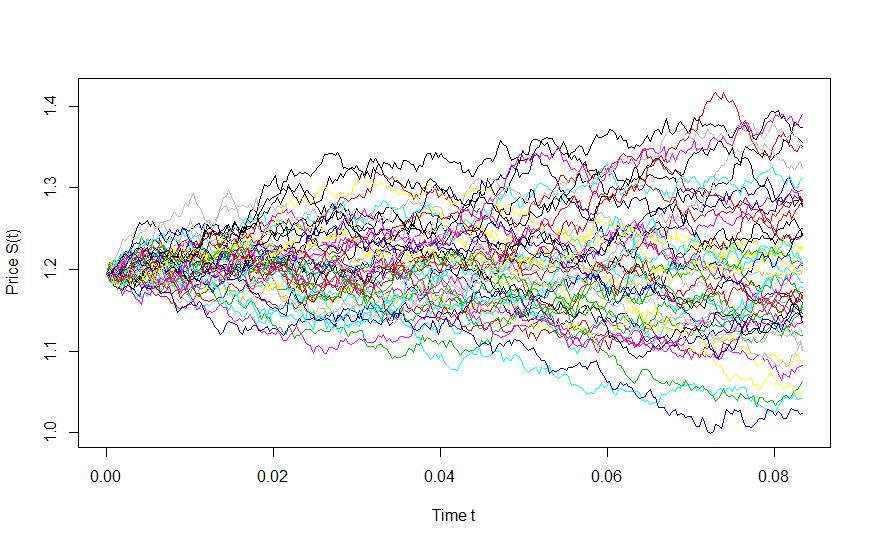
Did I mention that the famous Black Scholes options pricing formula also uses Brownian motion in its derivation with the assumption of constant volatility? As said above, volatility is not constant so we often see the options price to diverge from the price predicted by the Black Scholes options pricing formula with the famous smile effect. I am not going to go into the details of the derivation of Black Scholes options pricing formula here and describe how the stochastic volatility models solve the smile problem of Black Scholes formula.If you want to generate a few stock price sample paths you can use this R code below:
library(sde)
#define the return and volatility
mu=0.14
sigma=0.25
nt=50
n=2^8
#initial price
P0=1.19542
T=1/12
#generate Brownian motion sample paths of currency price
dt=T/n
t=seq(0,T,by=dt)
B= matrix(rep(0,length(t)*nt), nrow=nt)
for (i in 1:nt)
{
 B[i,]=GBM(x=P0,r=mu,sigma=sigma,T=T,N=n)

}

##plotting the Price Brownian motion sample paths
##boundary for the simulated price
ymax=max(B)
ymin=min(B)
plot(t,B[1,],t='l',ylim=c(ymin, ymax),col=1,ylab="Price S(t)",
     xlab="Time t")
for (i in 2:nt)
{
lines(t, B[i,], t='l', ylim=c(ymin, ymax),col=i)
}
}
I have posted the sample paths generated with this R code in the beginning of this post. Did you notice one thing in the stock price sample paths image, the stock price paths don’t have sudden jumps like that we do observe in the stock market or for that matter the currency market? Guess, what can be the reason? The reason is simple. We have assumed volatility and stock returns to be constant in the above R code that generated the stock price sample paths. As I have said before, constant volatility assumption made in Black Scholes options pricing formula has been found to be violated all the time by the market. So we cannot take volatility constant. Now let’s do something really interesting that most traders want to do but can’t do.
Trading Strategy Using Brownian Motion-How To Predict Stock Price High Low In A Certain Time?
We are traders. We want to develop trading strategies that can make money for us. Wall Street firms have got big pockets. These Wall Street firms employ MIT PhDs known as Quants. Quants develop sophisticated mathematical quantitative trading strategies. Forget technical analysis. Technical analysis is too subjective most of the time and has no statistical significance. Only that technical analysis works that is objective meaning if we cannot code a trading strategy, it is subjective and we cannot measure its winning ratio and do other statistical tests that can tell us how much robust our trading strategy is. Chart patterns are subjective most of the time. Subjective things have no scientific value. Let’s develop a quantitative trading strategy that can predict the high and low of currency pair price or for that matter stock price in the next 5 hours or 10 hours.
We have lot of high frequency financial time series data now available. All price data below daily timeframe is high frequency data. Daily and weekly and monthly data is known as low frequency data. We want to check if currency price is hit a certain level within this time. We cannot do it with technical analysis. Technical analysis gives many subjective methods but they are useless as most of the time they don’t work. This time we will use stochastic calculus and Brownian motion to predict whether price has a high chance of hitting a certain high or low in in the coming few hours that we define. Trading strategy is much more than a forecasting price. We need to precisely determine when to take action like buy and sell. So we have to do much more than forecasting price when developing a trading strategy. So a trading strategy should tell you when to open a buy/sell order with minimum risk and when to take profit and quit.
Our basic model uses the standard stock price model: $dS=\mu S dt + \sigma S dB_1$. We cannot assume volatility to be constant. So we need a second model for calculating volatility. As said above we assume volatility to be a random variable just like the stock price. Our volatility model equation is $d\sigma= p(S, \sigma, t)dt + q(S, \sigma,t)dB_2$. As said $B_1$ and $B_2$ are two correlated Brownian motions. $p(S, \sigma,t)$ and $q(S, \sigma,t)$ are two functions that we will need to estimate before we can make any meaningful predictions. Let’s take the logarithm of stock price and volatility $y_t = log( S_t )$ and $z_t = log( \sigma_t )$. With this transformation after using Ito Lemma we have the following dynamic state space continuous time model: $y_t = ( \mu_t – 1/2 \sigma_t ) dt + \sqrt{\sigma_t} dB_1$ and $dz_t = \kappa ( \theta – \sigma_t ) dt + \zeta \sqrt{\sigma_t} dB_2$.
We are using Heston Model keep this in mind. Sounds complicated? Well quantitative trading models are complicated. I just wanted to give you a taste of how much complicated mathematics is being used in today’s financial markets. You need a PhD in mathematics in order to understand and use the above formulas. I don’t have a PhD in mathematics but I can understand the above formula. I took one year to learn stochastic calculus. Now I know how to use this formula and develop a trading strategy. Continuing the discussion we need to discretize the above formula and then estimate it using Bayesian models. This is the discrete model that we can use: $ ln( S_t) = ln( S_{t-1} + ( \mu – 1/2 \sigma_t ) \Delta t + \sqrt{t} \sqrt{\sigma_t} B_t$ and the formula for calculating volatility is even a bit more complicated. We will now use Markov Chain Monte Carlo (MCMC) to build a particle filter that sequentially updates the whole formula on each new price tick. Sounds complicated?
You must know the concept of stopping time in a stochastic process that we need now to move further in our quantitative trading model. The aim of this quantitative trading strategy is to use high frequency price data to predict the high and low of the stock price or for that matter the currency pair price in the next couple of hours. Knowing the most probable levels where the price is going to reverse is going to skyrocket your trading profits. This is how the quants are making a killing on a daily basis while we retail traders look at the traditional support and resistance levels where price can turn. Most of the time price does not honor these traditional S/R levels. Quants have an edge. This edge is provided by their mathematical models and powerful computers that they use. Now don’t worry. You can run this quantitative trading strategy on your laptop or desktop if you have a GPU processor installed. Even a CPU processor can calculate this quantitative trading strategy. Why? Everything is done sequentially so we are only calculating the latest candle or what we call incorporating latest data in our Bayesian model.
Everything runs on a powerful computer so you have to build this quantitative trading model and code it only once. Once you have thoroughly tested it, you can use it to predict the price in the next few hours. This was just a glimpse of how Quants build their quantitative trading strategies. As a retail trader, you are competing against them. Trading is a zero sum game. Either you win and they lose or you lose and they win. The chances of you losing are high if you don’t take your trading strategies to the next higher level using quantitative finance. Keep reading my Forex Trading blog if you like this post as I will post more interesting articles on quantitative trading in the coming months.